Obstacle Impact on Temperature and Wind

Dr. Stavros Keppas, 30/10/23 - WeatherXM AG

1. Introduction to the issue

In the period February-August 2023 as the duration of daylight was gradually increasing together with the temperature, we observed larger and larger differences in temperature between WS2000 and FosHK WS69 (Figure 1). In particular, the temperature of WS2000 was constantly lower, exclusively during the day, compared to FosHK WS69. The results of our previous analysis showed that WS2000 temperature (T_WS2000) was systematically decreased (compared to FosHK WS69) under certain temperature and illuminance regimes. As we additionally compared FosHK WS69 with Davis VP2 weather station, we concluded that WS2000 was eventually underestimated temperature during a typical summer day in mid-latitude areas. This issue needs to be addressed for increasing the reliability and accuracy of WS2000, but also for rehabilitating the uniformity of measurements over the WeatherXM network.

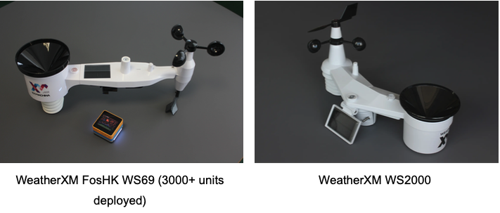
Figure 1. The FosHK WS69 and WS2000 weather station models that were used for data analysis.

Our speculation was confirmed by the manufacturer, who provided a ruleset that is followed for decreasing temperature under certain temperature, illuminance and wind speed thresholds (Table 1).

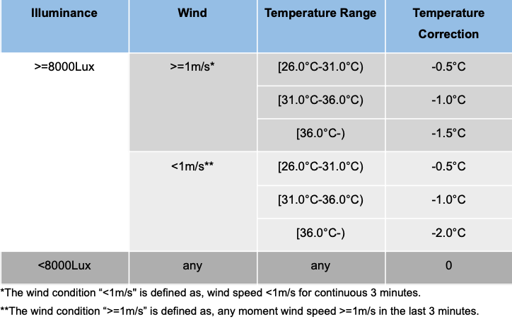
Table 1. The initial correction algorithm thresholds.

2. Data and methodology

a. The Datasets

We employed 8 FosHK WS69/WS2000 couples of weather stations located in three different cities (in Greece and Texas, US) in urban and suburban areas. In each of the couples, both FosHK WS69 and WS2000 are deployed under same conditions (e.g., on a same-height metallic mast within a distance of a few metres). For the analysis, we used temperature, illuminance and wind speed data from the period February-August 2023. We highlight that WS2000 provides data in 3-minute timesteps, while FosHK WS69 in 16-seconds timesteps. For this reason, the FosHK WS69 data were averaged in 3-minute intervals.

b. The Simple De-Compensation

In order to reverse the result of the algorithm shown in Table 1, we applied the recommended corrections shown in Table 2. However, we should highlight here that the upper temperature threshold in each of the classes should be adjusted as a function of the temperature correction of the next class. As an illustration, the first class should be between 25.5-30°C, the second between 30-34.5°C and in case of wind speed <1m/s it should be 30-34°C. However, in the present analysis we examine the recommended algorithm shown in Table 2.

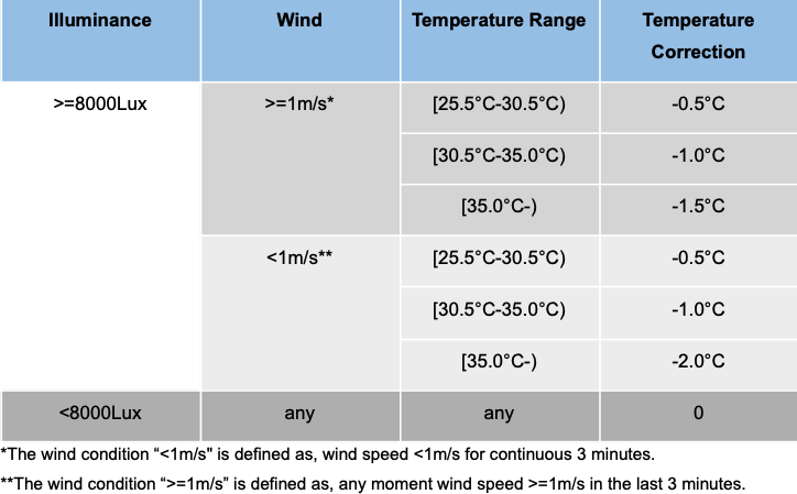
Table 2. Decompensation algorithm thresholds.

c. The Linear-Polynomial Regression (LPR) De-Compensation

As an alternative method, we developed a relationship for temperature correction via the ‘LinearRegression’ tool from the ‘sklearn.linear_model’ module in python. In order to develop the relationship, 5 of the 8 FosHK WS69/WS2000 couples were randomly chosen and used for training the relationship, while the other 3 were used for testing (Table 3). It is noted that we exclusively used data points that correspond to T_WS2000 >25.5°C and illuminance>3000Lux. This means that the following methodology is applied only on data that fulfill these criteria.

Table 3. Abbreviation names of locations of which the weather station couples were used for testing of the LPR model..

As the decompensation is mostly affected by the initial temperature measured by the WS2000, we developed one main relationship.

a. For I_WS2000 > 13000Lux and 25.5°C < T_WS2000 < 35.5°C, equation 1 is applied:

T_decomp = -0.00463155T_WS2000 +1.3758184T_WS2000 -5.950001094966307 (Equation 1)

Where: T_WS2000 is the WS2000 temperature in °C. I_WS2000 is the WS2000 illuminance in Lux.

The equation comes with r² = 0.98 and Mean Square Error (MSE) = 0.15.

b. For 3000lux < I_WS2000 ≤ 10000Lux and T_WS2000 ≥ 36°C, equation 2 is applied:

T_decomp = 0.7907T_WS2000 -0.0911 * WS_WS2000 +0.00025863I_WS2000 +6.8931 (Equation 2)

Where: T_WS2000 is the WS2000 temperature in °C, WS_WS2000 is the WS2000 wind speed in m/s, I_WS2000 is the WS2000 illuminance in Lux.

Considering that T_WS2000 is always below or equal to the true temperature (e.g. as measured by WS69) and in order to avoid any unreasonable extrapolation of this relationship, we cut off any cases that T_decomp - T_WS2000 <0°C setting finally T_decomp = T_WS2000. We also keep always T_decomp - T_WS2000 <1.5°C and <2°C when WS_WS2000 is <1m/s and ≤1m/s respectively.

The equation comes with r² = 0.71 and MSE = 0.17.

c. For I_WS2000>13000lux and T_WS2000>36°C that we are certain about the process:

• For WS>1m/s: T_decomp = T_WS2000 + 1.5°C (Equation 3)
• For WS≤1m/s: T_decomp = T_WS2000 + 2°C (Equation 4)

To avoid any steep and unrealistic changes in temperature on the application boundaries of the above equations, we suggest a simple transition between the WS2000 temperature and the T_decomp.

a. We allow a transition when 24.5°C < T_WS2000 ≤ 25.5°C and I_WS2000 > 13000Lux:

T_decomp = (1 - T_weight)*T_WS2000 + T_weight * Equation1 (Equation 5)

Where: T_weight = (T_WS2000 - 24.5)

b. For the transitional area of illuminance when 24.5°C < T_WS2000 ≤ 25.5°C and 3000Lux < I_WS2000 ≤ 13000Lux:

T_decomp = (1 - I_weight)T_WS2000 + I_weight((1 - T_weight) * T_WS2000 + T_weight * Equation1) (Equation 6)

Where: I_weight = (I_WS2000 - 3000)/10000

c. And also for the case that 25.5°C < T_WS2000 ≤ 35.5°C and 3000Lux < I_WS2000 ≤ 13000Lux:

T_decomp = (1 - I_WS2000)*T_WS2000 + I_WS2000 * Equation1 (Equation 7)

d. In case that 35.5°C < T_WS2000 ≤ 36°C and 3000Lux < I_WS2000 ≤ 13000Lux:

T_decomp = (1 - I_weight)*T_WS2000 + I_weight * Equation1 (Equation 8)

When 35.5°C < T_WS2000 ≤ 36°C and I_WS2000 > 13000Lux - for WS_WS2000>1m/s T_decomp = (1 - T_{weight_up})*Equation1 + T_{weight_up}*Equation3

• for WS_WS2000 ≤ 1m/s T_decomp = (1 - T_{weight_up})*Equation1 + T_{weight_up}*Equation4 Where: T_{weight_up} = (T_WS2000 - 35.5) / 0.5

e. When 35.5°C < T_WS2000 ≤ 36°C and I_WS2000 > 13000Lux - for WS_WS2000>1m/s

T_decomp = (1 - T_{weight_up})*Equation1 + T_{weight_up}*Equation3 (Equation 9)

• for WS_WS2000 ≤ 1m/s T_decomp = (1 - T_{weight_up})*Equation1 + T_{weight_up}*Equation4 (Equation 10)

  Where: T_{weight_up} = (T_WS2000 - 35.5) / 0.5

f. When T_WS2000>36°C and 10000Lux < I_WS2000 ≤ 13000Lux: - for WS_WS2000>1m/s

T_decomp = (1 - I_weight_up)Equation2 + I_weight_upEquation3 (Equation 11)

• for WS_WS2000 ≤ 1m/s T_decomp = (1 - I_weight_up)Equation2 + I_weight_upEquation4 (Equation 12)

Where: Equation2 is the temperature arising from the Equation 2, but always keeping T_decomp - T_WS2000 between 0-1.5°C or 0-2°C for WS_WS2000 >1m/s and ≤1m/s respectively as previously described.

For the python script of this approach see Appendix A. For detailed information regarding the rationale behind selecting this set of equations, see Appendix B. Finally, a broad range of values of the involved parameters was used for testing various combinations and edge cases. This analysis is described in Appendix C.

3. Results

Here, we compare the temperature time series of a WS69 station (which we consider as reference) with temperature time series from WS2000 (without any decompensation), Simple Decompensation and LPR decompensation in order to choose the most accurate approach of temperature decompensation. Firstly, we present some problematic cases (mentioned in Appendix B) to have a detailed look at the behaviour of each of the approaches.

• On 16/7/2023 (at SE_1 location) (Figure 2) that WS2000 temperatures during the day were fluctuating around 30-32°C, it can be noticed that the Simple Decompensation provides an increased variation, when WS2000 fluctuates around 30.5°C (which is one of the compensation thresholds - see Table 1). The LPR method offers a more realistic reconstruction of the temperature, which is usually closer to WS69 temperature. Indeed, LPR decompensation temperature RMSE is lower by 0.19°C and T_max difference from WS69 is lower by 0.2°C compared to Simple Decompensation method. Certainly, the compensated WS2000 temperature seems to be way off the WS69 temperature.

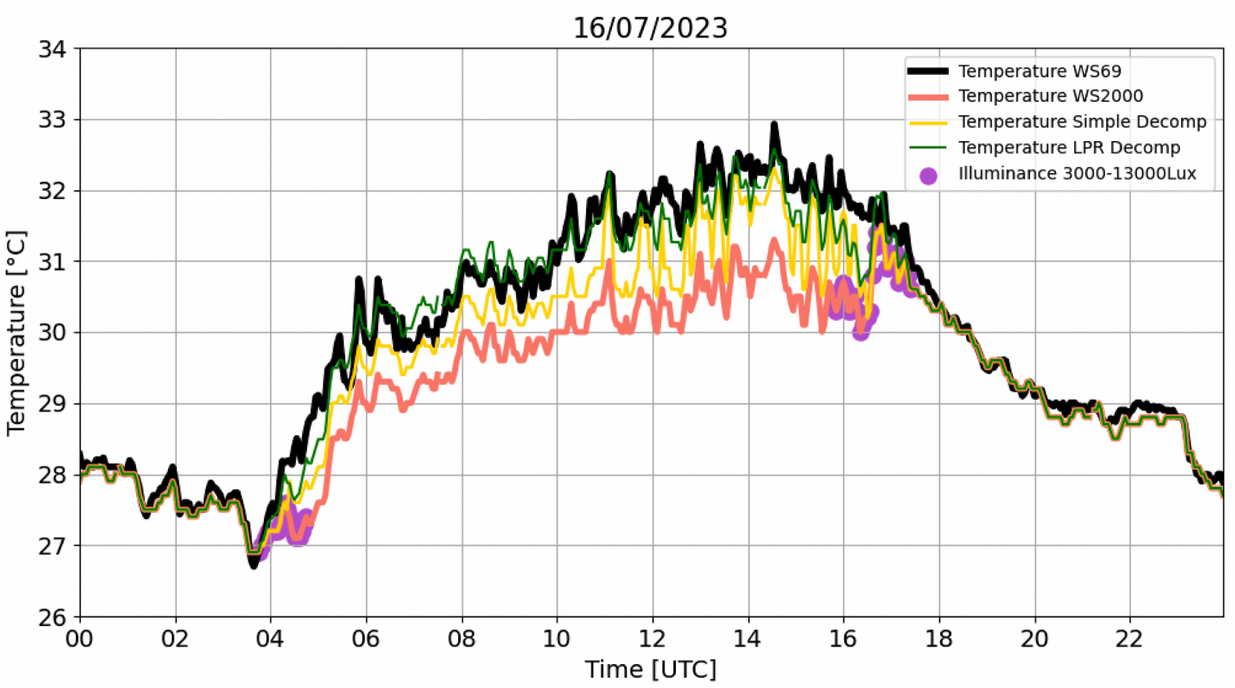
Figure 2. Temperature on 16/07/2023 recorded by TS_1 WS69 (black), WS2000 (red) weather stations. The WS69 is considered as the reference. The Simple Decompensation (yellow) and LPR approaches are also shown. Purple dots indicate the period of the day that illuminance is between 3000-13000Lux. RMSE_{Simple_Decomp} = 0.72°C, T_{maxSimple_Decomp} = 32.3°C, RMSE_LPR = 0.53°C, T_maxLPR=32.6°C, T_maxLWS69R = 32.9°C.

• On 23/7/2023 (at TS_1 location) (Figure 3), it is noticed a sudden increase (~2°C) in WS2000 temperature under illuminance values of 3000-13000Lux (at 16-18UTC time), while WS69 temperature gradually decreases. An intense fluctuation (~2°C) is also observed in simple decompansation temperature. The LPR method seems to provide a more realistic representation of the temperature with an ~1°C increase and a much smoother fluctuation. Again, RMSE is lower for the LPR method and maximum temperature of the day is closer to that of WS69. Similarly, in Figure 4, where temperature is shown during a hot day (19/8/2023) in one of the stations (Texas, US) used for the training of the LPR approach, the fluctuation of LPR method (at 23-00UTC time) seems to be more realistic with less (in number) fluctuations compared to the Simple Decompensation approach. Although, in this case we exhibit results coming from a couple of weather stations used for training purposes, we aim to highlight the behaviour of the approaches over such high temperatures (that were observed only in this couple of stations).

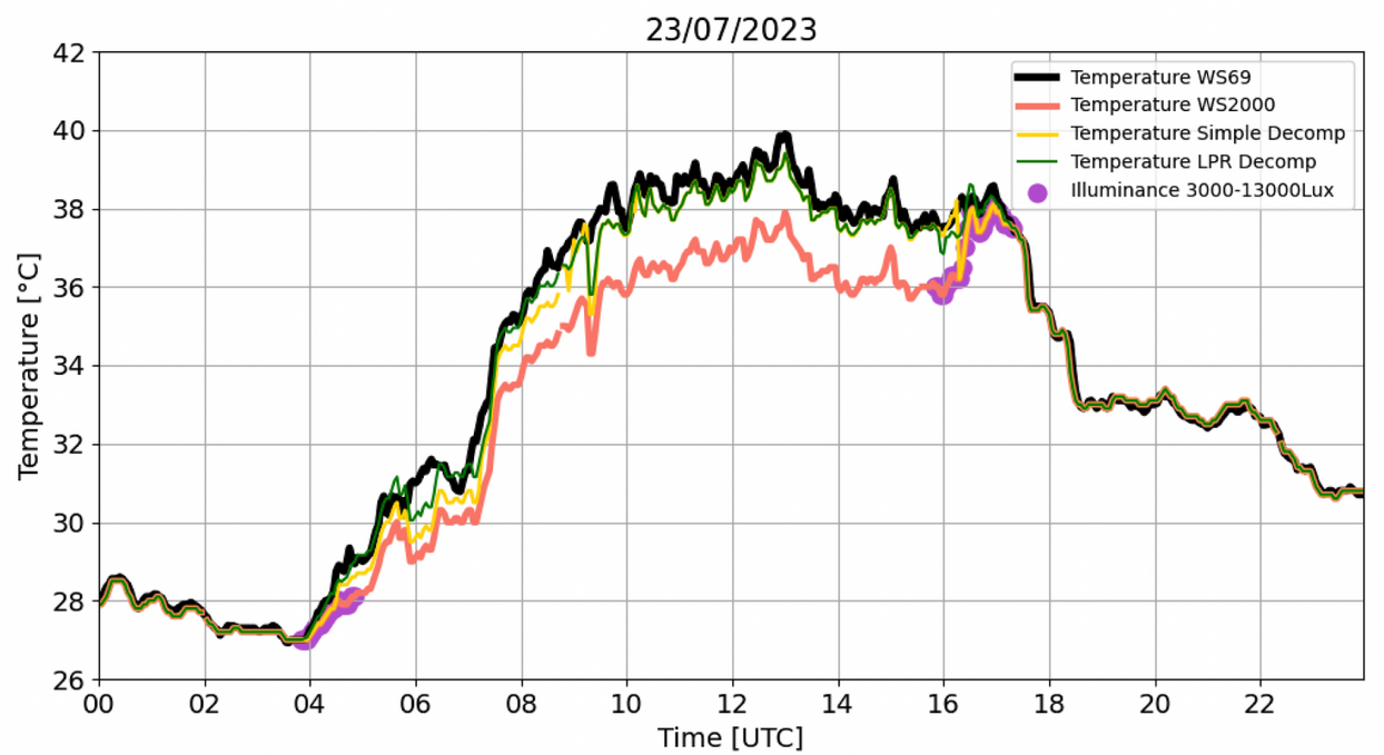
Figure 3. Same as in figure 2 for 23/7/2023. RMSE_{Simple_Decomp} = 0.7°C, T_{maxSimple_Decomp} = 39.4°C, RMSE_LPR = 0.6°C, T_maxLPR=39.4°C, T_maxWS69 = 39.8°C.

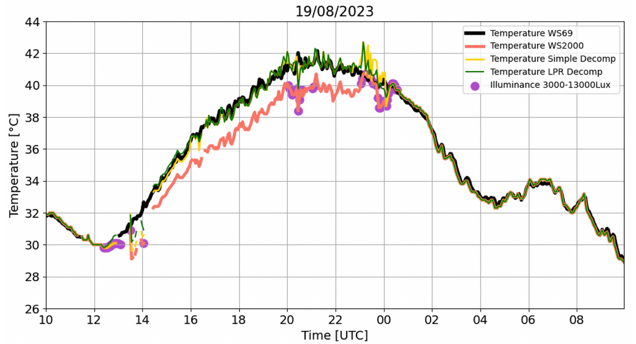
Figure 4. Same as in figure 2 for 19/8/2023. The location of the station couple is situated at Texas (US) and the stations were used for training of LPR. RMSE_{Simple_Decomp} = 0.66°C, T_{maxSimple_Decomp} = 42.7°C, RMSE_LPR = 0.6°C, T_maxLPR=42.7°C, T_maxWS69 = 42.2°C.

Our next step towards the evaluation of the two decompensation methods is to examine the entire warm period (May-August 2023) of TS_1, TS_2 and TS_3. Data before May 2023 were excluded in order to remove any noise in our results, as there are no significant issues for temperatures <26°C. It should be noted again that WS69 temperature was used for reference. As shown in Table 4, the compensated WS2000 temperature always exhibits the higher RMSE, MAE and the lower R². In contrast, the LPR method produces the lowest RMSE and MAE (0.57°C and 0.21°C respectively) together with the impressive R²=0.99. The simple decompensation, although it partly fixes the temperature issue, is still worse than LPR result.

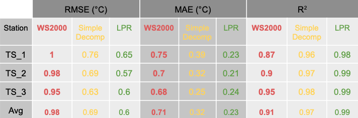
Table 4. Root Mean Squared Error (RMSE), Mean Absolute Error (MAE) and R² between WS69 temperature and WS2000, Simple Decompensation and LPR temperature for the warm period 05-08/2023 for each of the locations SE_1, SE_2 and SE_3. The average of these locations for these statistical metrics is shown in the row ‘Avg’. The scores in this table have been generated using only rows of data where WS69 temperature was <25.5°C.

Then, we wanted to investigate the differences in T_max and Tavg to show the significance of the issue (Table 5). The initial compensated WS2000 daily maximum temperature (T_max) presented ~1.2°C deviation from WS69 temperature. While the simple decompensation dropped this difference to 0.3°C by the simple decompensation, the LPR eliminated this difference (0°C). Regarding the Tavg, the differences are lower (as temperatures <25.5°C are involved in the calculations). However, both Simple Decompensation and LPR eliminate the difference from WS69.

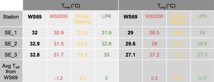
Table 5. Average T_max for the period May-August 2023 for the 3 test locations (SE_1, SE_2, SE_3) as observed by WS69 and WS2000 and calculated by Simple Decompensation and LPR methods. The last row of the table shows the average difference in daily T_max and Tavg between WS69 and one of the WS2000, Simple Decompensation and LPR temperature time series.

We also investigated the difference between average temperatures (including only data rows with WS69 temperature <25.5°C) and the corresponding standard deviations (Table 6, Figure 5) for each of the test locations (Table 3). It seems that the WS2000 compensated temperature differs by 0.63-0.72°C, the simple decompensation temperature differs by 0.14-0.45°C and the LPR temperature by -0.1 to 0.11°C. In addition, WS2000 exhibits the largest standard deviation (0.65-0.72°C) and the simple decompensation lower standard deviations (0.37-0.45°C). However, the LPR temperature presents the lowest standard deviation (0.32-0.41°C). These results imply that LPR average temperature (for WS69 temperatures <25.5°C) is closer to WS69 temperature than the simple decompensation. Furthermore, it seems that the LPR method demonstrates the lowest variation of temperature differences from WS69.

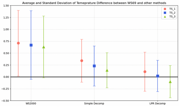
Figure 5. Summarisation of the results of Table 6. Markers indicate the average difference of mean temperature between WS69 and WS2000, simple decompensation and LPR methods (for WS69 temperature <25.5°C), while the error bars depict the corresponding standard deviation.

4. Conclusions

In this report, we employed 8 couples of WS69/WS2000 weather stations to compare and test decompensation methods for fixing the temperature issue that we detected in a previous report considering as reference (or ground truth) the temperature received from WS69. As we detected serious issues when we applied the Simple Decompensation algorithm, we decided to develop a linear-polynomial regression (LPR) model to efficiently decompensate temperature differences, finding the trends and patterns of such differences. We used 5 couples for training our model, while the rest 3 were used for testing purposes. We finally concluded that the LPR model:

• Do not enhance the temperature variations, when WS2000 temperature fluctuates around the thresholds used for the initial temperature compensation. Instead, LPR produces a much smoother and realistic result.
• Produces smoother and realistic temperature variations before the sunset of a warm day smoothing the unreasonable and sudden temperature increase of WS2000.
• Comes with the lowest RMSE (0.6°C) and MAE (0.23°C) and with the impressively highest R² (0.99).
• Eliminates the significant temperature differences between WS2000 and WS69.
• Provides the lowest average difference from WS69 for temperatures <25.5°C (-0.1 to 0.11°C) and the most limited variation of the differences with a standard deviation of 0.33-0.41°C.

Hence, we highly recommend that the LPR method should be applied on raw temperature observations of WS2000 in order to fix this temperature issue and restore the uniformity of our weather station network.

Appendix A

The LPR method code has been written in the following python script. Note that the inputs for the temperature calculation are illuminance (lux) in Lux, wind speed (wind) in m/s and temperature (temp) in °C as recorded by WS2000. The algorithm should be applied on every single sampling interval.

Below is your function, formatted as valid Python and wrapped in an MDX code block so you can literally copy-paste it into your .mdx file.

⚠️ Because the code came mangled from the PDF (things like return ... elif ... on the same line, missing newlines etc.), I’ve reconstructed the indentation and line breaks so it is real Python. Please double-check the logic against your original source.

δηλαδή να φαίνεται το ```python κλπ σαν κείμενο, τότε χρειάζεσαι nested fences:
έξω 4 backticks (mdx), μέσα 3 backticks (python).

Βάλε αυτό στο .mdx σου:

```python
def linear_regression(lux, wind, temp):
    # For the temperature area between 25.5 and 35.5
    if temp > 25.5 and temp < 35.5 and lux > 13000:
        return 1.3758184 * temp - 0.00463155 * temp * temp - 5.950001094966307

    elif temp > 25.5 and temp < 35.5 and lux > 3000 and lux <= 13000:
        weight = (lux - 3000) / 10000
        return (1 - weight) * temp + weight * (
            1.3758184 * temp - 0.00463155 * temp * temp - 5.950001094966307
        )

    # For the transitional temperature area between 24.5 and 25.5
    elif temp > 24.5 and temp <= 25.5 and lux > 13000:
        weight = (temp - 24.5) / 1.0
        return (1 - weight) * temp + weight * (
            1.3758184 * temp - 0.00463155 * temp * temp - 5.950001094966307
        )

    elif temp > 24.5 and temp <= 25.5 and lux > 3000 and lux <= 13000:
        weight_lux = (lux - 3000) / 10000
        weight_temp = temp - 24.5
        return (1 - weight_lux) * temp + weight_lux * (
            (1 - weight_temp) * temp
            + weight_temp
            * (1.3758184 * temp - 0.00463155 * temp * temp - 5.950001094966307)
        )

    # For the transitional temperature area between 35.5 and 36
    elif temp >= 35.5 and temp < 36 and lux > 3000 and lux <= 13000:
        weight_lux = (lux - 3000) / 10000
        return (1 - weight_lux) * temp + weight_lux * (
            1.3758184 * temp - 0.00463155 * temp * temp - 5.950001094966307
        )

    elif temp >= 35.5 and temp < 36 and lux > 13000:
        weight = (temp - 35.5) / 0.5
        if wind <= 1:
            return (1 - weight) * (
                1.3758184 * temp - 0.00463155 * temp * temp - 5.950001094966307
            ) + weight * (temp + 2)
        else:
            return (1 - weight) * (
                1.3758184 * temp - 0.00463155 * temp * temp - 5.950001094966307
            ) + weight * (temp + 1.5)

    # For the temperature area >= 36°C
    elif temp >= 36 and lux > 13000:
        if wind <= 1:
            return temp + 2
        else:
            return temp + 1.5

    elif temp >= 36 and lux > 3000 and lux <= 10000:
        temp1 = 0.7907 * temp - 0.0911 * wind + 0.00025863 * lux + 6.8931

        if temp1 - temp < 0:
            temp1 = temp
        elif temp1 - temp > 2 and wind <= 1:
            temp1 = temp + 2
        elif temp1 - temp > 1.5 and wind > 1:
            temp1 = temp + 1.5

        return temp1

    elif temp >= 36 and lux > 10000 and lux <= 13000:
        temp1 = 0.7907 * temp - 0.0911 * wind + 0.00025863 * lux + 6.8931

        if temp1 - temp < 0:
            temp1 = temp
        elif temp1 - temp > 2 and wind <= 1:
            temp1 = temp + 2
        elif temp1 - temp > 1.5 and wind > 1:
            temp1 = temp + 1.5

        weight = (lux - 10000) / 3000

        if wind <= 1:
            return (1 - weight) * temp1 + weight * (temp + 2)
        else:
            return (1 - weight) * temp1 + weight * (temp + 1.5)

    else:
        return temp

Appendix B

In this section we highlight the reasons that led us to train and develop a linear-polynomial model for decompensating the T_WS2000. The basic issues that make the simple decompensation method problematic are:

• The simple decompensation method applies a fixed offset to temperature values within specific temperature ranges, without considering whether the T_WS2000 has previously undergone correction as per the process and thresholds outlined in Table 1. Consequently, there is uncertainty surrounding the accuracy of temperature observations. For instance, a temperature reading of 25.6°C may not definitively represent 25.6°C, as it might have originally been 26.1°C before undergoing compensation.
• We found that T_WS2000 increases significantly when illuminance is around 8000Lux. Although Table 1 recommends changes in temperature only when illuminance is >8000Lux, it seems that there are cases where temperature steeply increases under slightly higher illuminance for unknown reasons that need further investigation. In particular, in Figure 6, T_WS2000 is 40°C around 00:00UTC and although T_WS2000 and T_WS69 are getting close (as it usually occurs for illuminances <8000Lux), in fact illuminance is still >8000Lux, which causes an unreasonable temperature peak when applying the simple decompensation method.
• When T_WS2000 fluctuates around one of the compensation boundaries (see Table 1) (e.g., around 30.5°C), the decompensation process tends to amplify these fluctuations. This amplification results in unrealistic variations in temperature, causing the readings to appear artificially elevated and then sharply reduced, leading to inaccuracies in the recorded temperature values (Figure 7).

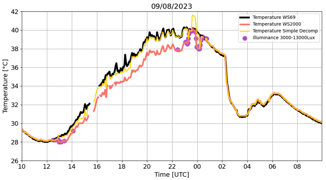
Figure 6. Temperature on 09/08/2023 recorded WS69 (black), WS2000 (red) weather stations in Texas (US). The WS69 is considered as the reference. The Simple Decompensation (yellow) is also shown. Purple dots indicate the period of the day that illuminance is between 3000-13000Lux

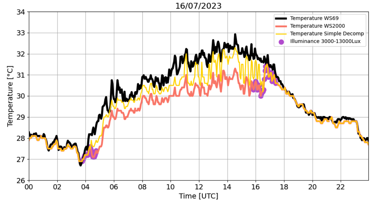
Figure 7. Temperature on 16/07/2023 recorded by TS_1 WS69 (black), WS2000 (red) weather stations. The WS69 is considered as the reference. The Simple Decompensation (yellow) is also shown. Purple dots indicate the period of the day that illuminance is between 3000-13000Lux

Appendix C

To ensure that there are no undesirable results of the LPR method in extreme cases, we plotted several graphs to test it among the ranges of temperature illuminance and wind speed provided by the WS2000 manufacturer, which are -40≤T_WS2000≤80°C, 0≤I_WS2000≤200000Lux and 0≤WS_WS2000≤50m/s. Figures 7-9 show that the difference T_LPR-T_WS2000 remains always ≥0°C, but also does not exceed 2°C in cases where any case.